Quantitative approach to floods and flooding

Quantitative approach to floods and flooding
by Dr. Eric M. Baer, Geology Program, Highline Community CollegeFloods and flooding quantitatively
Discharge, stage, flood stage, and crest: What's
the difference?
Rating a river: the relationship between
discharge and stage
Flood stage and inundation area: it's not just how
high the river is
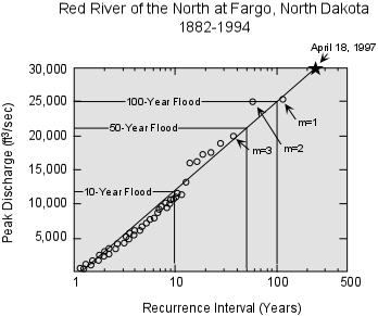
What is a one hundred year flood?
Flood forecasting: forecasts based on historic data
and the "100-year flood"
An example of taking historical discharges to
forecasted inundations
Resources and activities
Quantitiative approach to floods and flooding
Essential Concepts
Generally there are five main concepts that our students struggle with when thinking about floods:
- the various ways that we measure the size or flow of a river,
- the relationship between discharge and stage,
- how a rise in flood stage leads to an area of inundation,
- flood forecasts, probabilities, recurrence intervals and how to calculate them,
- the meaning of a "100-year flood".
Discharge
Discharge, stage, flood stage, and crest: What's the difference?
Students often get confused by the variety of ways the size or magnitude of flows in rivers are measured and communicated. It is not that these concepts are difficult, however if these terms are not explicitly defined, students often end up perplexed.
- Discharge is the volume of water that passes through a given cross section per unit time, usually measured in cubic feet per second (cfs) or cubic meters per second (cms).
- Stage is the level of the water surface over a datum (often sea level). As discharge increases, stage increases, however the relationship is not linear.
- Flood stage is the stage at which overbank flows are of sufficient magnitude to cause considerable inundation of land and roads and/or significantly threaten life and property. Students often confuse this with overbank flow which is when water overtops the channel and has geomorphic impacts.
- Crest (or peak) is the highest stage reached during a hydrologic event (such as a flood).
In class, and for most hydrologic needs, the discharge (also called flow) is the critical measure of the river. However, it is difficult to measure discharge, so the most common way flows are reported in the media is by stage. In the case of a flood, news reports will often say that a river is "5 feet above flood stage". Floods and rivers also have a crest which is often reported in relationship to flood stage as in "the river will crest at 7 feet above flood stage tomorrow."
Rating a River
Rating a river: the relationship between discharge and stage
The relationship between discharge and stage is empirical and typically is represented graphically as a rating curve.

Rating curve for the Connecticut River at Montague City station
The making of a rating curve is difficult, but is crucial to taking measurements (like stage) and turning them into the much more useful discharge information. Ideally, I would take students out to a stream a couple of times and have them measure discharge and stage so they get an idea of these measurements (see Discharge and Sediment Transport in the Field for an example). That is usually not possible, so I lead an open ended discussion of how we can measure the discharge. I start out with the definition of discharge and then have them come up with the methods they would use. I then have them think about how, if they made that measurement multiple times over many years they could develop a rating curve. Rating curves are an excellent topic for class discussion because they often seem simple to students at first glance, but are much more complicated. I often ask things like "what happens to a river when the discharge increases?" and then have students explore the rather complicated answers. For example, rating curves may change with time and there is often significant scatter in the data, which can be used as a launching point for discussing regressions and error.
Flood stage and inundation area: it's not just how high the river is
Often students have a difficult time realizing that the area of inundation for a flood depends not just on the stage, but also on the slope of the ground around the water. This is often expressed as students:
- wanting the flood to spread a fixed distance from the stream, independent of topographic changes
- viewing floods as primarily a lateral movement of water rather than a vertical change in the water level (they sometimes think they will get pushed perpendicular to the flow instead of downstream)
I often have students do a couple of cross-sections along differing parts of the stream/river so as to illustrate that the aerial extent of flood inundation is dependent on the topography of the stream channel.
For some students that really have a hard time visualizing inundation area as a function of topography, I have an inexpensive model of a stream made from a plastic food storage container and modeling clay. I have one stream channel narrow and steep sided and the other broad and relatively flat. I then pour water into the model to simulate the rise of water from a flood and see the difference in inundation area. In the steep valley they can see that the flood does not spread far away from its original channel whereas in the broader valley the area under water is much greater.
The impact of a flood that raises the water level of a stream by 10 feet is very dependent on the slopes of the valley. In a steep canyon, there might be no significant impact, while on a broad flood plain the water could cover a great area and do tremendous damage. So the damage in a flood is not only dependent on the discharge, but also the topography around a river. In fact, engineers often build levees to artificially steepen the sides of a river in order to reduce flood damage.
Flood forecasting: forecasts based on historic data and the "100-year
flood"
Flood forecasts are determined by examining past occurrences of flooding events, determining recurrence intervals of historical events, and then extrapolating to future probabilities. These calculations are often very difficult for students to understand because of the use difficult graphs to extrapolate data. Typically, the maximum annual discharge is examined and ranked to generate a recurrence interval for historical discharges. The calculations needed to make these forecasts are discussed on the recurrence interval page and the probability pages.
The determination of recurrence intervals has many inherent assumptions that are often false. One assumption is that each flood event is independent of previous flooding events, which is often false. Another assumption is that the occurrences and recurrence intervals of floods in the past is the same as the occurrences in the future. Because drainage basins are changed by human activities and other events, and rainfall may be changing due to local or global climate variations, the extrapolation of past events to the future may be invalid.
Once the recurrence intervals of historic data are determined, these are plotted on graph paper in order to extrapolate to events beyond the historical record. Many exercises use log-normal graph paper to make this graph. However, this assumes a log-normal distribution of flood data when there are many possible distributions including log-normal, Gumbel, and Pearson distributions. A correct (at least according to the U.S. government) manner of determining flood frequency is to do a Log-Pearson Type III analysis.
> To learn more about flood frequency distributions, you may want to look at Flood frequency distributions, a .pdf file of a U.S.G.S. document describing various distributions and how to fit them to data or at Log-Pearson Type III analysis, a web page that has step-by step instructions on how to do this analysis for stream data using excel. The extrapolations of recurrence intervals are then to forecast the future probability of a flood of a given discharge.
The probability (P) of an flood with recurrence interval T is
P = 1/T
An example of taking historical discharges to forecasted inundations

Rating curve for the Raging River The town of Wetsfield sits on the Raging River. They are planning to install a new sewage treatment plant and want to know where to put it. Concerned by potential damage from floods, they decide that they need to examine several proposed sites for flood risk. They first gather data from a local stream gauge which shows the maximum annual stage each year. Unfortunately, the gauge has only been operating for 16 years. They then assign a recurrence interval to each of the year’s peak floods.
| Year | discharge | ranking | RI |
|---|---|---|---|
| 2004 | 134 | 3 | 5.666667 |
| 2003 | 119 | 8 | 2.125 |
| 2002 | 118 | 9 | 1.888889 |
| 2001 | 137 | 2 | 8.5 |
| 2000 | 111 | 14 | 1.214286 |
| 1999 | 125 | 5 | 3.4 |
| 1998 | 114 | 12 | 1.416667 |
| 1997 | 111 | 15 | 1.133333 |
| 1996 | 171 | 1 | 17 |
| 1995 | 117 | 10 | 1.7 |
| 1994 | 130 | 4 | 4.25 |
| 1993 | 121 | 7 | 2.428571 |
| 1992 | 123 | 6 | 2.833333 |
| 1991 | 115 | 11 | 1.545455 |
| 1990 | 112 | 13 | 1.307692 |
| 1989 | 110 | 16 | 1.0625 |
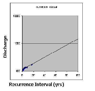
Graph for projecting recurrence intervals on the Raging river
To find out the stage of such floods, the town consults the Raging river's rating curve. They find that the 25 year flood discharge would be at about 700 feet elevation, while the 50 year flood would be at 710 feet elevation and the 100 year flood would be at 730 feet elevation. So if they site the treatment plant at 730 feet, they would have a 1 percent chance any given year of the plant being flooded.
What is a one hundred year flood?
The term "a one-hundred year flood" is actually a misnomer, and as a result causes a great deal of confusion with students and professionals alike. What is really meant by this term is a flood with recurrence interval of 100 years - one that has a 1% chance of occurring in any given year. There are several ideas and resources for teaching recurrence intervals for floods and other events on the recurrence interval page.
Understanding odds and probability in the geosciences
Jump down to:
Strategies | Materials & Exercises | Resources
Probability is the study of the chance that a particular event or series of events will occur. Typically, the chance of an event or series of events will occur is expressed on a scale from 0 (impossible) to 1 (certainty) or as an equivalent percentage from 0 to 100%.
The probability (Pf) of a favorable outcome is

Pf = f/n
-
where:
- n is the total number of possible outcomes and
- f is the number of possible outcomes that match the favorable outcome criteria.
Strategies: Ideas from Mathematics
Put quantitative concepts in context

- Hazard assessment including earthquakes, floods , and volcanic eruptions
- Extinctions and extinction rates
- Error and data analysis (including uncertainty and error propagation)
- Forecasting
Use multiple representations
Because everyone has different ways of learning, mathematicians have defined a number of ways that quantitative concepts can be represented to individuals. Here are some ways that probabilities can be represented.
Verbal representation Probabilities are often given verbally as a percentage, such as a "50% chance." Other times probabilities are even represented by qualitative terms such as "sure," "unlikely," or "almost certain." For example,
The U.S weather service defines several verbal probabilities:
- slight chance - 20% probability
- chance - 30-50 % probability
- likely - 60-70 % probability
- no qualifier - 80-100% probability
Numerical representation One common source of confusion is that probabilities are represented in many differing ways all of which mean the same thing. Probabilities can be represented as a ratio, percentage, fraction or as a decimal; I often point this out to students, so they are alert to the multiple ways we represent odds. This often brings up difficulties and fears with basic mathematics including fractions, percentages and ratios.
Some ways of representing the same probability
- ratio - written as 1:3 or 1 in 3.
- fraction - 1/3 or sometimes even as an unreduced fraction 3/9
- percentage - 33%
- decimal - 0.33
Tabular representation Tables are often used to show probabilities across a sample space, called a probability distribution.
| Sum | probability (fractional) | probability (percentage) |
| 2 | 1/36 | 2.78% |
| 3 | 2/36 | 5.56% |
| 4 | 3/36 | 8.33% |
| 5 | 4/36 | 11.11% |
| 6 | 5/36 | 13.89% |
| 7 | 6/36 | 16.67% |
| 8 | 5/36 | 13.89% |
| 9 | 4/36 | 11.11% |
| 10 | 3/36 | 8.33% |
| 11 | 2/36 | 5.56% |
| 12 | 1/36 | 2.78% |
| TOTAL | 36/36 | 100% |
Graphical representation There are several graphical ways to portray both probabilities and probability distributions.
Graphical ways of showing probabilities
 Bar
Bar 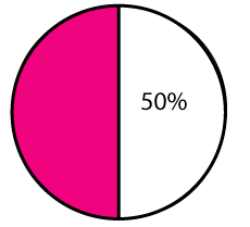 Pie chart
 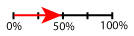 Number line
 Graphical ways of showing probability distributions
Bar chart 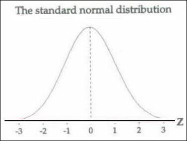 Distribution probability
 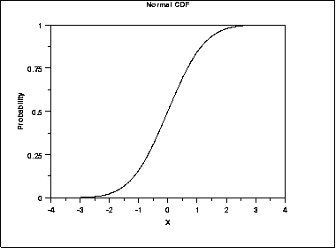 Cumulative percent
 Model representation There are many models one can use as an introduction to probability, including dice rolls, coin tosses, causes of death, and chances of floods.
One example is the probability of death due to individual causes. For instance, a typical American has a one in three chance of dying in a heart attack, a one in 1/100 chance of being killed in auto accident and an estimated 1 in 20,000 chance of being killed by a meteor strike. These probabilities can then be used to stimulate a discussion if geologic hazards, impact of risk perceptions, and mathematical calculations of probability.
Chance/probability of death from various causes for an average American in a given year.
| Cause of death | Probability |
|---|---|
| Aids/HIV infection | 1 in 19,000 |
| Airplane Crash | 1 in 2,736,000 |
| Alcoholic Liver Disease | 1 in 22,000 |
| Car Crash | 1 in 6357 |
| Earthquake | 0 to 1 in 40,000,000 |
| Falls | 1 in 20,688 |
| Flood | 1 in 6,700,000 |
| Food Poisoning | 1 in 53,000 |
| Heart disease | 1 in 387 |
| Homicide | 1 in 16439 |
| Suicide | 1 in 9350 |
Algebraic representation The probability (Pf) of a favorable outcome is
-
Pf = f/n
Use technology appropriately

Students have any number of technological tools that they can use to better understand quantitative concepts -- from the calculators in their backpacks to the computers in their dorm rooms. Probability and recurrence intervals can make use of these tools to help the students understand this often difficult concept.
Graphing calculators
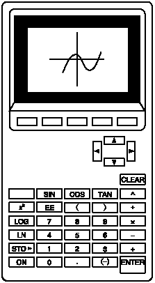
Graphing calculators are an easy way for all students to enter data and to see what a curve of that data looks like. All graphing calculators are slightly different and students may need help with their particular model.
Computers

Probability provides an excellent opening for an introduction to the use of spreadsheet programs. Spreadsheet programs can be used to develop probability distributions and to generate graphs of these distributions. An example to start with might be the probability of rolling a particular sum for 1, 2, 3 and more sets of dice. Students are likely to encounter spreadsheet programs in many of their classes and they are excellent tools for visualizing the shape of an equation.
Work in groups to do multiple day, in-depth problems

Mathematicians also indicate that students learn quantitative concepts better when they work in groups and revisit a concept on more than one day. Therefore, when discussing quantitative concepts in entry-level geoscience courses, have students discuss or practice the concepts together. Also, make sure that you either include problems that may be extended over more than one class period or revisit the concept on numerous occasions.
Probability is a concept that comes up over and over in introductory geoscience: Volcanic eruptions, mass extinctions, earthquakes, floods, confidence intervals, etc. When each new topic is introduced, make sure to point out that they have seen this type of mathematics before and should recognize it.
Recurrence intervals
by Dr. Eric M. Baer, Geology Program, Highline Community CollegeJump down to:
randomness | forecasting vs. recurrence | how to calculate | materials exercises
Essential Concepts
Generally, there are four concepts that our students struggle with when studying recurrence intervals:
- the concept of a recurrence interval
- the idea that random events that are independent of previous events
- the difference between recurrence intervals and forecasting
- how to calculate recurrence intervals when data have variable magnitudes and when they don't.
Recurrence interval
When geologic events are random or quasi-random, it is helpful to represent their frequency as an average time between past events, a "recurrence interval" also known as a "return time." For instance, there have been 7 subduction zone earthquakes in the Pacific Northwest in the past 3500 years, giving a recurrence interval of about 500 years.How do geologists use this concept?
Recurrence intervals occur in a variety of geologic contexts including:
- flood frequency
- earthquake hazards
- volcanic eruption frequency
- severe weather and storms
- meteor impacts
These many contexts occur throughout an introductory geoscience course and give opportunities to revisit and reinforce this concept.
What is meant by "random"?
Random events have a probability of occurring that do not depend on the past. While this may not always be true, for many geologic events this is a robust model. For more information on teaching and using probability, please look at our probability page.
Students express their misunderstanding of random events in a variety of ways:
- People often talk of events being "due," usually when the time without an event exceeds the recurrence interval.
- Students think that because an event has occurred recently it cannot happen again.
- Even clearly random events are often not perceived as truly random; many people are convinced that streaks exist ("the dice are hot so I should keep going") or in luck ("I have lost the last 10 times, so my luck HAS to change.") These superstitions may be transferred to geologic processes.
To reinforce the idea that geologic events are random, I often relate them to events that they recognize as random such as flipping a coin or rolling a 6 on a die. When we talk about streaks, I use the question "how does the die/coin know what it rolled the last time?" as a way to dispel misperceptions arising out of superstitions. Students can also see this by conducting an experiment flipping coins. I have each student flip a coin until they get three heads or tails in a row. Then I have the entire class flip one more time. They see that half of the class that continues their "streak" and half breaks their "streak."
Recurrence intervals vs. forecasting
Recurrence intervals refer to the past occurrence of random events. Forecasting refers to the future likelihood of random events. These are often confused because the recurrence interval (calculated from past events) is used to gauge the future probability of an event. However, the mathematics used with these two concepts are very different. The confusion between the past-determined recurrence interval and the forecasted probability is reinforced by the widespread use of "a 100-year flood" to mean a "flood with a 1% probability of occurring in any given year."
Recurrence intervals
Determination of the recurrence interval is straight-forward when looking at past events. Where there is no associated magnitude or a limited magnitude (such as pumice-producing volcanic eruptions) the recurrence interval (T) is the number of events (N) divided by the number of years in the record (n). An example of an activity using these calculations is Determining Earthquake Probability and Recurrence.
T = N/n
T = (n+1)/m
Student activities using these calculations are
Two streams, two stories... How Humans Alter Floods and Streams
and
Flood Frequency and Risk Assessment.
The Los Angeles River at Sepulveda Blvd had the following peak discharges between 1970 and 1979 (data from the U.S.G.S.):
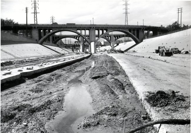
The L.A. River at Sepulveda Blvd
| Year | Discharge (cfs) |
|---|---|
| 1970 | 81,806 |
| 1971 | 123,006 |
| 1972 | 75,806 |
| 1973 | 112,006 |
| 1974 | 99,706 |
| 1975 | 114,006 |
| 1976 | 57,406 |
| 1977 | 95,106 |
| 1978 | 147,006 |
| 1979 | 112,006 |
The data can be reorganized, and a recurrence interval computed for each discharge. In this case, n is 10, because we are using 10 years of data.
| Year | Discharge | rank (m) | recurrence interval (n+1)/m |
|---|---|---|---|
| 1976 | 57,406 | 10 | 1.1 |
| 1972 | 75,806 | 9 | 1.2 |
| 1970 | 81,806 | 8 | 1.4 |
| 1977 | 95,106 | 7 | 1.6 |
| 1974 | 99,706 | 6 | 1.83 |
| 1973 | 112,006 | 5 | 2.2 |
| 1979 | 112,006 | 4 | 2.8 |
| 1975 | 114,006 | 3 | 3.7 |
| 1971 | 123,006 | 2 | 5.5 |
| 1978 | 147,006 | 1 | 11 |
Note that these are not the true recurrence values for the L.A. River since only a selection of available data have been used.
Forecasting
Once we start looking to the future, we are looking at forecasting which is governed by the mathematics of probability. The probability (P) of an event with recurrence intervalT
-
is
P = 1/T
PT
PT = 1 – Pr
Illustrating the difference between forecasts and intervals
A flood is a 100-year flood if the discharge has exceeded that value on average once every 100 years in the past. In this case the probability of such a flood occurring in the next year is 1/100 or 1%. Many students would assume that the chance of a 100-year flood occurring in the next 100 years is 100%, but that is not true. It may be counter-intuitive to students that that a 100-year flood has a less than two thirds chance of occurring in 100 years. I explain that the chance of a 100-year flood not happening in the next 100 years is 99%100, or 36.6%. If the probability of an event NOT happening is 36.6%, the probability of it happening is 63.4%. I also explain that that there is a chance that 2 or even 3 100-year events will occur within a given 100 year period. As a result, the average recurrence will drop from these more closely spaced events. Indeed, there is only about a 35% chance that a single 100-year flood will occur in 100 years, an 18% chance that 2 100-year floods will occur, and even a nearly 2% chance that we will get four 100-year events within a given 100 year time period.
Resources and activities
- Two streams, two stories... How Humans Alter Floods and Streams In this exercise, students look at data from two streams in the Seattle metro area. They calculate the 100-year flood on each stream for two different time periods and note the changes wrought by urbanization and damming. This is designed to be worked in groups and can be done in-class or at home.
- Chemung River Flood Recurrence Intervals. A WWW and spreadsheet-based exercise on flood-frequency analysis, from the Journal of Geoscience Education, v. 46, 1998. In MS Word form.
- Flood
Frequency
and Risk Assessment In this lab, students calculate recurrence
intervals for various degrees of flooding on a portion of the Des
Moines River in Iowa, based on historical data. Then they plot these
calculations on a flood frequency curve. Combining flood frequency
data with a topographic map of the region, students do a risk
assessment for the surrounding community.
- Rethinking Flood Prediction: Why the Traditional Approach Needs to
Change Gosnold, W. D., et al., 2000. , Geotimes, v. 45, n. 5, p.
20-23. This article, not freely available on-line, discusses many of
the problems with flood forecasting.
- Discharge and Sediment Transport in the Field In this field activity, students collect field data on channel geometry, flow velocity, and bed materials. Using these data, they apply flow resistance equations (Manning and the depth slope product) and sediment transport relations (Shields curve) to estimate the bankfull discharge and to determine if the flow is sufficient to mobilize the bed. This activity requires students to utilize theoretical and empirical equations derived in class in the context of a field problem.
Resources
- Information from FEMA about flood hazards and mitigation
- Floods and floodplains contains general background information on floods.
- Significant Floods in the United States During the 20th Century - USGS Measures a Century of Floods lists thirty-two of the most significant floods (in terms of number of lives lost and (or) property damage) in the United States during the 20th century according to the various types of floods. Internet sites for acquiring near-real-time streamflow data and other pertinent flood information are provided.
- The "1OO-Year Flood" explains how and when uncommon big floods happen.
- You can view up-to-date information on national flood-threat forecast from the National Weather Service and NOAA.
- Water resources in the United States from the U.S.G.S. This is an entry site into many resources including water data regional studies and more.
- Water resources data from the U.S.G.S. This page provide access to water-resources data collected at more than 1 million sites in all 50 States, the District of Columbia, and Puerto Rico.
Probability
- Determining
Earthquake
Probability and Recurrence In this exercise students gather real
web-based data on earthquakes in the Pacific Northwest, calculate
recurrence intervals on these events and make estimations of
recurrence intervals on future events. Includes analysis of error and
societal implication discussions. Designed as a combination in-class
and web-based homework assignment. This could easily be altered to
look at earthquake possibilities for any geographic area.
- Chance news This site contains materials to help teach a Chance course. Chance is a quantitative literacy course. It includes "The Chance News" a newsletter that includes lesson plans and articles with discussion questions from the Chance magazine. A source for supplementary material for teaching or introducing basic probability.
- The Math Forum has extensive links to classroom resources. Look in Exploring Data for finding and displaying data sets. Also included are an Internet Mathematics Library, Course Materials & Lesson Plans, Collections of Course Materials & Lesson Plans, Problems and Puzzles, Probability and statistics software, internet projects, and Reference Materials