Radioactive Dating
Radioactive Dating
principle sources: Australian Museum https://australianmuseum.net.au/the-geological-time-scaleWikipedia https://en.wikipedia.org/wiki/Radiometric_dating
Carleton University http://serc.carleton.edu/research_education/geochemsheets/techniques/gassourcemassspec.html
Radioactive Isotopes - the "Clocks in Rocks" Numerical and Relative Ages for Rocks
Overview Geological Time
How is Geological Time Measured?
Geological Divisions
Time Related Terms
Radiometric Dating
Half-life - Parent Daughter Isotopes
Parent Decay and
Daughter Growth Curves
Re-setting the Clock - Closure
Temperature
Radio Carbon Dating
Dating the Rocks with Sr-Rb "Isochron" Method
What steps are involved in Rb-Sr Dating?
A Mass Spectrometer is used to Measure
Isotopic Ratios
More Parent-Daughter Relationships
Thermoluminescence Dating
see also Geological time...
see also Dendrochronlolgy...
see
also Carbon 14 Date Calculator
Overview Geological Time
A numerical (or "absolute") age is a specific number of years, like 150 million years ago. A relative age simply states whether one rock formation is older or younger than another formation. The Geologic Time Scale was originally laid out using relative dating principles.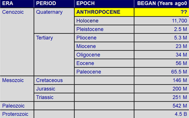
The geological time scale is based on the the geological rock record, which includes erosion, mountain building and other geological events. Over hundreds to thousands of millions of years, continents, oceans and mountain ranges have moved vast distances both vertically and horizontally. For example, areas that were once deep oceans hundreds of millions of years ago are now mountainous desert regions.
How is geological time measured?
The earliest geological time scales simply used the order of rocks laid down in a sedimentary rock sequence (stratum) with the oldest at the bottom. However, a more powerful tool was the fossilised remains of ancient animals and plants within the rock strata. After Charles Darwin's publication Origin of Species (Darwin himself was also a geologist) in 1859, geologists realised that particular fossils were restricted to particular layers of rock. This built up the first generalised geological time scale.Once formations and stratigraphic sequences were mapped around the world, sequences could be matched from the faunal successions. These sequences apply from the beginning of the Cambrian period, which contains the first evidence of macro-fossils. Fossil assemblages 'fingerprint' formations, even though some species may range through several different formations. This feature allowed William Smith (an engineer and surveyor who worked in the coal mines of England in the late 1700s) to order the fossils he started to collect in south-eastern England in 1793. He noted that different formations contained different fossils and he could map one formation from another by the differences in the fossils. As he mapped across southern England, he drew up a stratigraphic succession of rocks although they appeared in different places at different levels.
By matching similar fossils in different regions throughout the world, correlations were built up over many years. Only when radioactive isotopes were developed in the early 1900s did stratigraphic correlations become less important as igneous and metamorphic rocks could be dated for the first time.
Geological divisions
Divisions in the geological time scales still use fossil evidence and mark major changes in the dominance of particular life forms. For example, the Devonian Period is known as the 'Age of Fishes', as fish began to flourish at this stage. However, the end of the Devonian was marked by the predominance of a different life form, plants, which in turn denotes the beginning of the Carboniferous Period. The different periods can be further subdivided (e.g. Early Cambrian, Middle Cambrian and Late Cambrian).
This is the latest version of the time scale, as revised and published in 2012.
| Era | Period | Epoch | Start/End |
|---|---|---|---|
| Archaean | 4.56 - 2.5 billion years ago | ||
| Proterozoic | 2.5 billion - 541 million years ago | ||
| Palaeozoic |
Cambrian | 541 - 485 million years ago | |
| Ordovician | 485 - 444 million years ago | ||
| Silurian | 444 - 419 million years ago | ||
| Devonian | 419 - 359 million years ago | ||
| Carboniferous | 359 - 298 million years ago | ||
| Permian | 298 - 252 million years ago | ||
| Mesozoic |
Triassic | 252 - 201 million years ago | |
| Jurassic | 201 - 145 million years ago | ||
| Cretaceous | 145 - 65 million years ago | ||
| Cenozoic | Palaeocene | 66 - 56 million years ago | |
| Eocene | 56 - 34 million years ago | ||
| Oligocene | 34 - 23 million years ago | ||
| Miocene | 23 - 5.3 million years ago | ||
| Pliocene | 5.3 -2.6 million years ago | ||
| Quaternary | Pleistocene | 2.6 million -10,000 years ago | |
| Holocene | 10,000 years ago to the present |
Time Related Terms
- Faunal succession: is the time arrangement of fossils in the geological record.
- Formations: are stratigraphic successions containing rocks of related geological age that formed within the same geological setting.
- Ga: is an abbreviation used for billions (thousand million) of years ago.
- Geochronology: is the study of the age of geological materials.
- Ma: is an abbreviation used for millions of years ago.
- Palaeobiology: is the study of the evolution of life during geologic time.
- Palaeobotany: is the study of ancient plants.
- Palaeontology: is the study of ancient lifeforms.
- Stratigraphic succession: is a sequence of layered sedimentary rocks.

Radiometric (Radioactive) Dating
The basic equation of radiometric dating requires that neither the parent nuclide nor the daughter product can enter or leave the material after its formation. The possible confounding effects of contamination of parent and daughter isotopes have to be considered, as do the effects of any loss or gain of such isotopes since the sample was created. It is therefore essential to have as much information as possible about the material being dated and to check for possible signs of alteration.[8] Precision is enhanced if measurements are taken on multiple samples from different locations of the rock body. Alternatively, if several different minerals can be dated from the same sample and are assumed to be formed by the same event and were in equilibrium with the reservoir when they formed, they should form an isochron. This can reduce the problem of contamination. In uranium-lead dating, the concordia diagram is used which also decreases the problem of nuclide loss. Finally, correlation between different isotopic dating methods may be required to confirm the age of a sample. For example, the age of the Amitsoq gneisses from western Greenland was determined to be 3.6 ± 0.05 million years ago (MA) using uranium-lead dating and 3.56 ± 0.10 Ma using lead-lead dating, results that are consistent with each other.
Accurate radiometric dating generally requires that the parent has a long enough half-life that it will be present in significant amounts at the time of measurement (except as described below under "Dating with short-lived extinct radionuclides"), the half-life of the parent is accurately known, and enough of the daughter product is produced to be accurately measured and distinguished from the initial amount of the daughter present in the material. The procedures used to isolate and analyze the parent and daughter nuclides must be precise and accurate.
This normally involves isotope ratio mass spectrometry.
The precision of a dating method depends in part on the half-life of the radioactive isotope involved. For instance, carbon-14 has a half-life of 5,730 years. After an organism has been dead for 60,000 years, so little carbon-14 is left that accurate dating can not be established. On the other hand, the concentration of carbon-14 falls off so steeply that the age of relatively young remains can be determined precisely to within a few decades.
Half-Life - Parent and Daughter Isotopes
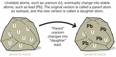
Numerical dating takes advantage of the "clocks in rocks" - radioactive isotopes ("parents") that spontaneously decay to form new isotopes ("daughters") while releasing energy.
For example, decay of the parent isotope Rb-87 (Rubidium) produces a stable daughter isotope, Sr-87 (Strontium), while releasing a beta particle (an electron from the nucleus). ("87" is the atomic mass number = protons + neutrons.
Numerical ages have been added to the Geologic Time Scale since the advent of radioactive age-dating techniques.
Many minerals contain radioactive isotopes.
In theory, the age of any of these minerals can be determined by:
1) counting the number of daughter isotopes in the mineral, and
2) using the known decay rate to calculate the length of time required to produce that number of daughters.
It illustrates how the amount of a radioactive parent isotope decreases with time. This amount is a percentage of the original parent amount. Time is expressed in half-lives. Experiment by dragging on the graph. For example when 42% of the parent still remains, 1.23 Half-Lives of time has passed.
Parent Decay and Daughter Growth Curves
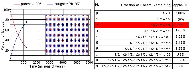
The half-life of U-235 decaying to Pb-207 is 713 million years. Note that this half-life can be obtained from the graph at the point where the decay and growth curves cross. Determine the half-lives for the other three isotopes and enter your estimate into the text fields below each graph. Note the differences in scale between the various graphs
Re-setting the Clock - Closure temperature
If a material that selectively rejects the daughter nuclide is heated, any daughter nuclides that have been accumulated over time will be lost through diffusion, setting the isotopic "clock" to zero. The temperature at which this happens is known as the closure temperature or blocking temperature and is specific to a particular material and isotopic system. These temperatures are experimentally determined in the lab by artificially resetting sample minerals using a high-temperature furnace.
As the mineral cools, the crystal structure begins to form and diffusion of isotopes is less easy. At a certain temperature, the crystal structure has formed sufficiently to prevent diffusion of isotopes. This temperature is what is known as closure temperature and represents the temperature below which the mineral is a closed system to isotopes.
Thus an igneous or metamorphic rock or melt, which is slowly cooling, does not begin to exhibit measurable radioactive decay until it cools below the closure temperature. The age that can be calculated by radiometric dating is thus the time at which the rock or mineral cooled to closure temperature. Dating of different minerals and/or isotope systems (with differing closure temperatures) within the same rock can therefore enable the tracking of the thermal history of the rock in question with time, and thus the history of metamorphic events may become known in detail.
This field is known as thermochronology or thermochronometry.
Radiocarbon Dating

The radiocarbon dating method was developed in the 1940's by Willard F. Libby and a team of scientists at the University of Chicago. It subsequently evolved into the most powerful method of dating late Pleistocene and Holocene artifacts and geologic events up to about 50,000 years in age. The radiocarbon method is applied in many different scientific fields, including archeology, geology, oceanography, hydrology, atmospheric science, and paleoclimatology. For his leadership, Libby received the Nobel Prize in Chemistry in 1960. See.. our C14 dating calculator
Dating Rocks with the Rb-Sr "Isochron" Method
There are numerous radioactive isotopes that can be used for numeric dating. All of the dating methods rely on the fundamental principles of radioactive decay, but the specific materials that can be dated and the exact procedures for calculating a date are very different from one method to the next.
The Rb-Sr method.
Rubidium occurs in nature as two isotopes: radioactive Rb-87 and stable Rb-85. Rb-87 decays with a half-life of 48.8 billion years to Sr-87. This half-life is so long that the Rb-Sr method is normally only used to date rocks that are older than about 100 million years.
Which minerals and rocks can be dated with the Rb-Sr method? The minerals must contain Rb, which is a rather rare element. Fortunately, Rb behaves chemically very much like the more common potassium (K), so that most K-bearing minerals contain a small amount of Rb. Examples include the mica family (biotite and muscovite) and the feldspar family (plagioclase and orthoclase). These minerals are abundant in granite (an igneous rock) and gneiss (a metamorphic rock).
What steps are involved in Rb-Sr dating?
- 1. Select a fresh, unweathered rock sample.
Sample Selection
A geologist collects a fresh, unweathered hand sample for age dating. Fresh is the key word here, and means that the chemistry of the sample has NOT been changed since the sample formed. Weathering alters the chemistry of rocks including their isotopic compositions. Therefore, a highly weathered rock may yield unreliable age information. - 2. Crush the rock and separate the Rb-bearing minerals.
Getting a Rock Sample Ready for the Mass Spectrometer
For reliable age determination, careful sample preparation is an important and often tedious process. The rock is mechanically crushed into small fragments. Fragments of the Rb-bearing minerals are then separated from the whole rock using a variety of methods, such as a magnetic separator. These materials are then used to prepare a "whole-rock" sample and several "mineral separate" samples. The whole rock sample will yield the weighted average isotopic composition of all the minerals in the rock. Each mineral separate will yield the composition of that particular mineral.
Other Steps
There are other steps that must be carried out to prepare a sample for analysis by a mass spectrometer, such as converting the sample to a solution by dissolving the mineral separates in selected acids, using techniques of column chemistry to increase the concentration of the small amounts of Rb and Sr in the solution and then precipitating the concentrated solution as a "salt" compound. It's this compound of Rb-Sr salts that can be attached to a special filament and placed into the mass spectrometer for analysis.
3. Analyze the isotopic compositions of the whole rock and mineral separates on a mass spectrometer.
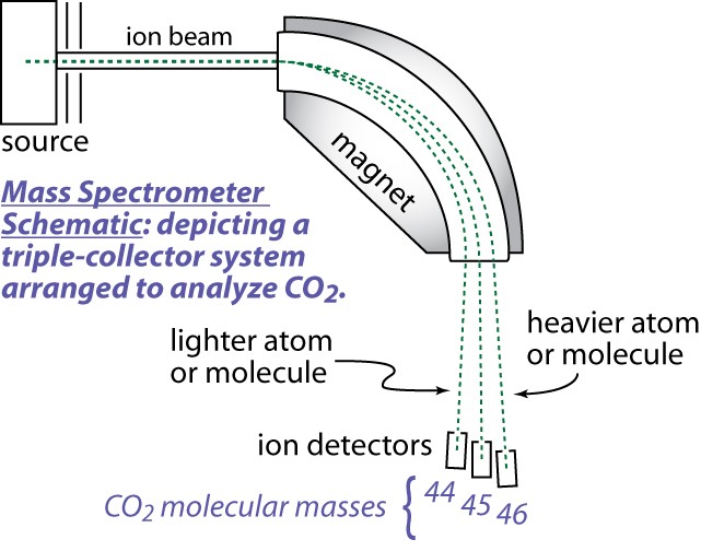
A Mass Spectrometer is used to Measure Isotopic Ratios
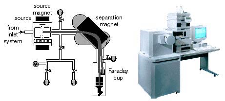
The gas source mass spectrometer includes three fundamental parts,
- (1) a "source" of positively charged ions or molecular ions,
- (2) a magnetic analyzer, and (3) ion collectors. The source is a low-pressure chamber (~10-5 torr) into which sample or standard gas is ionized, either by an electron beam produced by a hot filament, or by a strong electrostatic field. Once formed, the ions are accelerated and focused by charged plates into a beam that enters a flight tube. The flight tube has a bend that coincides with an electromagnet that alters the path of the ions according to their mass/charge ratio, thus several beams leave the magnetic sector. Multiple ion detectors are arranged to collect the ion beams of interest. These collectors measure each beam as a current that can be amplified and determined with high precision.
A Mass Spectrometer is a very powerful and sophisticated instrument. Many types exist. Below is a simplified diagram of the electro-mechanical mass spectrometer system and a picture of a modern instrument. Understanding how a mass spectrometer functions is beyond the level of this activity. But you should know that it measures the amounts of various isotopes present in specially prepared samples of rocks and minerals as well as other materials.
Understanding the isochron diagram is the key to determining the age of a rock using the Rb-Sr method.
More Parent-Daughter Relationships
Thermoluminensnce
Thermoluminescence (TL) dating is the determination, by means of measuring the accumulated radiation dose, of the time elapsed since material containing crystalline minerals was either heated (lava, ceramics) or exposed to sunlight (sediments).
As a crystalline material is heated during measurements the process of thermoluminescence starts. Thermoluminescence emits a weak light signal that is proportional to the radiation dose absorbed by the material. It is a type of luminescence dating.
Sediments are more expensive to date. The destruction of a relatively significant amount of sample material is necessary, which can be a limitation in the case of artworks.
The heating must have taken the object above 500° C, which covers most ceramics, although very high-fired porcelain creates other difficulties. It will often work well with stones that have been heated by fire. The clay core of bronze sculptures made by lost wax casting can also be tested.
Different materials vary considerably in their suitability for the technique, depending on several factors. Subsequent irradiation, for example if an x-ray is taken, can affect accuracy, as will the "annual dose" of radiation a buried object has received from the surrounding soil. Ideally this is assessed by measurements made at the precise findspot over a long period. For artworks, it may be sufficient to confirm whether a piece is broadly ancient or modern (that is, authentic or a fake), and this may be possible even if a precise date cannot be estimated.
Natural crystalline materials contain imperfections: impurity ions, stress dislocations, and other phenomena that disturb the regularity of the electric field that holds the atoms in the crystalline lattice together. These imperfections lead to local humps and dips in the crystalline material's electric potential. Where there is a dip (a so-called "electron trap"), a free electron may be attracted and trapped.
The flux of ionizing radiation—both from cosmic radiation and from natural radioactivity excites electrons from atoms in the crystal lattice into the conduction band where they can move freely. Most excited electrons will soon recombine with lattice ions, but some will be trapped, storing part of the energy of the radiation in the form of trapped electric charge Depending on the depth of the traps (the energy required to free an electron from them) the storage time of trapped electrons will vary as some traps are sufficiently deep to store charge for hundreds of thousands of years.
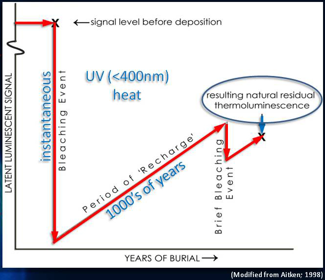
In thermoluminescence dating, these long-term traps are used to determine the age of materials: When irradiated crystalline material is again heated or exposed to strong light, the trapped electrons are given sufficient energy to escape. In the process of recombining with a lattice ion, they lose energy and emit photons (light quanta), detectable in the laboratory.
The amount of light produced is proportional to the number of trapped electrons that have been freed which is in turn proportional to the radiation dose accumulated. In order to relate the signal (the thermoluminescence—light produced when the material is heated) to the radiation dose that caused it, it is necessary tocalibrate the material with known doses of radiation since the density of traps is highly variable.
Thermoluminescence dating presupposes a "zeroing" event in the history of the material, either heating (in the case of pottery or lava) or exposure to sunlight (in the case of sediments), that removes the pre-existing trapped electrons. Therefore, at that point the thermoluminescence signal is zero. As time goes on, the ionizing radiation field around the material causes the trapped electrons to accumulate. In the laboratory, the accumulated radiation dose can be measured, but this by itself is insufficient to determine the time since the zeroing event.